Selecting a matched subsample
This is a second post in a series on splitting samples. In this case, say you have a very small sub-group of a large sample. You want to look at that subgroup and controls, but you don’t want your sample to be 90% controls. Instead, you want the subgroup and a sub-sample of controls matched on some demographic variables. As a further complication, lets make one variable (age) continuous, and lets make age and sex correlated with subgroup membership. This example is heavily cribbed from a post by Norbert Köhler.
library(sn)
library(tidyverse); library(ggthemes); theme_set(theme_tufte())
library(ggExtra)
library(pander)
library(MatchIt)
library(simstudy)
Simulation
set.seed(31453)

simdef<-defData(varname="age",
                dist="uniformInt",
                formula="120;144") #age in months between 10-12
simdef<-defData(simdef,varname="sex",
                dist="binary",
                formula=".5")
simdef<-defData(simdef,varname="parent.ed",
                dist="categorical",
                formula=genCatFormula(n=6))
simdef<-defData(simdef,varname="missingdata",
                dist="binary",
                formula=".2")
simdef<-defData(simdef,varname="inSubGroup",
                dist="binary",
                formula=".005/12 * (age-132) + .005*sex + .0175")


df<-genData(12000,simdef)

df$income<-rsn(nrow(df),alpha=3)
numbers_of_bins = 10
df <- df %>%
    mutate(
        # bin i:
        i.bin = cut(income,
                    breaks = unique(quantile(
                        income,
                        probs = seq.int(0, 1, by = 1 / numbers_of_bins)
                    )),
                    include.lowest = TRUE,
                    labels=FALSE)
    )

df<-as.data.frame(df)

factorialize<-c("sex","missingdata","parent.ed","inSubGroup")
df[factorialize] <- lapply(df[factorialize], factor)
levels(df$inSubGroup)<-c("control","treatment")

pander(head(df))
| id | age | sex | parent.ed | missingdata | inSubGroup | income | i.bin |
|---|---|---|---|---|---|---|---|
| 1 | 128 | 0 | 4 | 1 | control | 1.392 | 9 |
| 2 | 138 | 1 | 5 | 0 | control | -0.02661 | 1 |
| 3 | 130 | 1 | 6 | 0 | control | 1.911 | 10 |
| 4 | 127 | 1 | 5 | 0 | control | 0.3791 | 4 |
| 5 | 121 | 0 | 5 | 0 | control | 0.909 | 7 |
| 6 | 132 | 1 | 1 | 0 | control | 1.695 | 10 |
pander(table(df$inSubGroup))
| control | treatment |
|---|---|
| 11761 | 239 |
Is there an imbalance?
We only need to match on age, sex, and one other categorical variable.
imbalance_model <-
    matchit(
        inSubGroup ~ age +sex + i.bin,
        data = df,
        method = NULL,
        distance = "glm"
    )

summary(imbalance_model)
##
## Call:
## matchit(formula = inSubGroup ~ age + sex + i.bin, data = df,
##     method = NULL, distance = "glm")
##
## Summary of Balance for All Data:
##          Means Treated Means Control Std. Mean Diff. Var. Ratio eCDF Mean
## distance        0.0202        0.0199          0.1269     0.9939    0.0346
## age           132.4812      131.8617          0.0850     1.0289    0.0266
## sex0            0.4686        0.5021         -0.0671          .    0.0335
## sex1            0.5314        0.4979          0.0671          .    0.0335
## i.bin           5.3096        5.5039         -0.0672     1.0122    0.0195
##          eCDF Max
## distance   0.0856
## age        0.0600
## sex0       0.0335
## sex1       0.0335
## i.bin      0.0367
##
##
## Sample Sizes:
##           Control Treated
## All         11761     239
## Matched     11761     239
## Unmatched       0       0
## Discarded       0       0
Yes, age and sex are imbalanced (which we simulated). So is income!
Nearest Neighbor Matching
Note that it is important to code variable type correctly, i.e. that factors are factors and not numeric.
Sub-sampling
We want 2 controls per ‘treatment’ participant.
matching_model <-
    matchit(
        inSubGroup ~ age + sex + i.bin,
        data = df,
        method = "nearest",
        distance = "glm",
        ratio= 2
    )

summary(matching_model,un=FALSE)
##
## Call:
## matchit(formula = inSubGroup ~ age + sex + i.bin, data = df,
##     method = "nearest", distance = "glm", ratio = 2)
##
## Summary of Balance for Matched Data:
##          Means Treated Means Control Std. Mean Diff. Var. Ratio eCDF Mean
## distance        0.0202        0.0202               0     1.0021         0
## age           132.4812      132.4812               0     1.0021         0
## sex0            0.4686        0.4686               0          .         0
## sex1            0.5314        0.5314               0          .         0
## i.bin           5.3096        5.3096               0     1.0021         0
##          eCDF Max Std. Pair Dist.
## distance        0               0
## age             0               0
## sex0            0               0
## sex1            0               0
## i.bin           0               0
##
## Sample Sizes:
##           Control Treated
## All         11761     239
## Matched       478     239
## Unmatched   11283       0
## Discarded       0       0
The distribution parameters should be similar, and the control n should be twice the treated n. Then we save the new data frame:
df.match<-match.data(matching_model)[,1:ncol(df)]
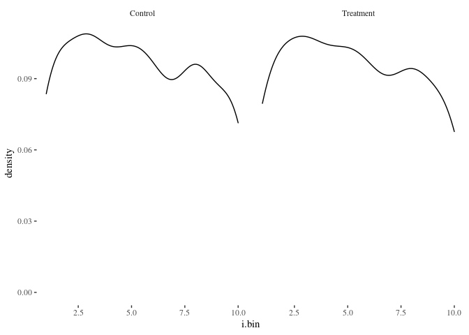
Checking
df.match$inSubGroup<-factor(df.match$inSubGroup,labels=c("Control","Treatment"))
histbygroup<-function(plotdata,xvar="i") {
    ggplot(plotdata,aes_string(x=xvar)) +
        geom_density() +
        facet_grid(~inSubGroup)
}

histbygroup(df.match,"i.bin")
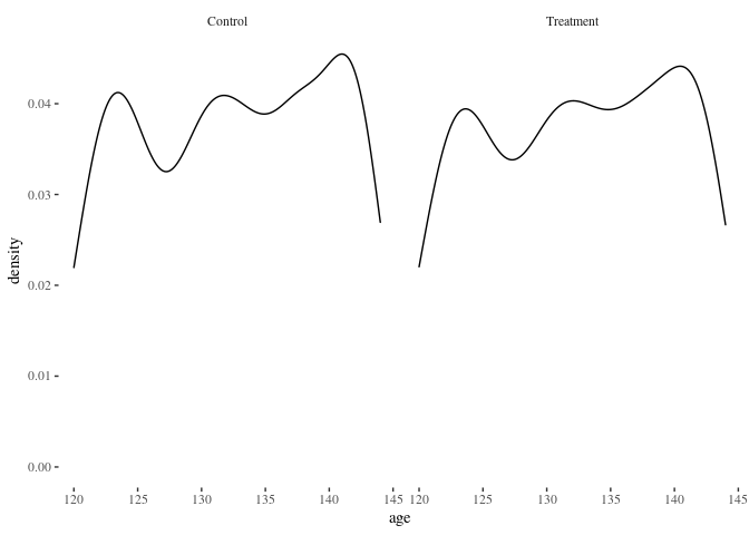
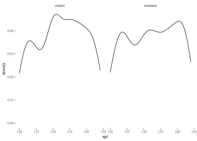
histbygroup(df.match,"age")
barbygroup<-function(plotdata,xvar="i") {
ggplot(plotdata,aes_string(x=xvar)) +
geom_bar() +
facet_grid(~inSubGroup)
}
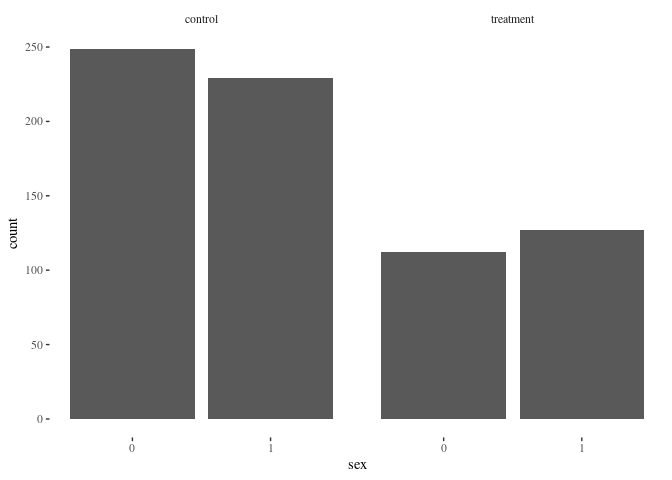
barbygroup(df.match,"sex")
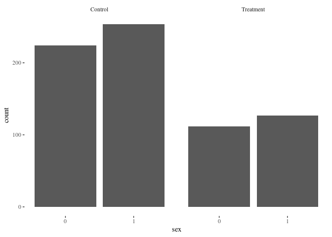
Nearest neighbor is doing pretty well! Here’s another method for comparison:
Optimal Matching
Sub-sampling
We want 2 controls per ‘treatment’ participant.
matching_model2 <-
    matchit(
        inSubGroup ~ age + sex + i.bin,
        data = df,
        method = "optimal",
        distance = "glm",
        ratio= 2
    )

summary(matching_model2,un=FALSE)
##
## Call:
## matchit(formula = inSubGroup ~ age + sex + i.bin, data = df,
##     method = "optimal", distance = "glm", ratio = 2)
##
## Summary of Balance for Matched Data:
##          Means Treated Means Control Std. Mean Diff. Var. Ratio eCDF Mean
## distance        0.0202        0.0201          0.0546     1.0202    0.0177
## age           132.4812      132.3891          0.0126     1.0956    0.0176
## sex0            0.4686        0.5209         -0.1048          .    0.0523
## sex1            0.5314        0.4791          0.1048          .    0.0523
## i.bin           5.3096        5.2573          0.0181     1.0224    0.0073
##          eCDF Max Std. Pair Dist.
## distance   0.0607          0.2131
## age        0.0460          0.7938
## sex0       0.0523          0.7085
## sex1       0.0523          0.7085
## i.bin      0.0167          0.9767
##
## Sample Sizes:
##           Control Treated
## All         11761     239
## Matched       478     239
## Unmatched   11283       0
## Discarded       0       0
The distribution parameters should be similar, and the control n should be twice the treated n. Then we save the new data frame:
df.match2<-match.data(matching_model2)[,1:ncol(df)]
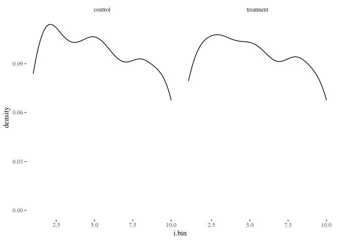
Checking
histbygroup<-function(plotdata,xvar="i") {
    ggplot(plotdata,aes_string(x=xvar)) +
        geom_density() +
        facet_grid(~inSubGroup)
}

histbygroup(df.match2,"i.bin")
histbygroup(df.match2,"age")
barbygroup<-function(plotdata,xvar="i") {
    ggplot(plotdata,aes_string(x=xvar)) +
        geom_bar() +
        facet_grid(~inSubGroup)
}

barbygroup(df.match2,"sex")
Nearest neighbor appears to do a better job